Binary Search Trees
AVL tree
B-Trees
Binary Search Trees
<<Introduction>>
heap의 한계
heap 자료구조는 root를 검색할 때만 O(logn)의 성능을 갖는다.
만약에 다른 item을 찾는 경우라면, O(n)의 시간 복잡도를 갖게 된다.
binary search tree의 필요성
균일하게 tree 높이에 비례한 시간복잡도 O(log2n)을 갖는 자료 구조이기 때문이다.
Binary search tree의 정의
전제 : 중복되는 요소가 없음
left sub-tree nodes < root < right sub-tree nodes가 재귀적으로 모든 트리에 적용됨
<<functions>>
search a key
구현 1. 재귀 함수
    def rBST(self, root, key):
        if not root:
            # 요소를 찾지 못한 경우
            return None
        if key == root.data:
            return root
        if key < root.data:
            return self.rBST(root.left)
        else:
            return self.rBST(root.right)
=> 시간 복잡도 : O(log2n) + recursion overhead
구현 2. 반복문
    def iBST(self, root, key):
        while root:
            if key == root.data:
                return root
            elif key < root.data:
                root = root.left
            else:
                root = root.right
        return None
=> 시간 복잡도 : O(log2n)
Insert
step 0. overlap check : 빈 트리이거나, 이미 해당 원소가 존재하는 경우
step 1. 마지막 원소와 new node를 비교한다.
    def insert(self, item):
        node = Node(item)
        # 빈 트리면, self.tree에 node를 할당해준다.
        if not self.tree:
            self.tree = node
        else:
            # 현재 노드
            temp = self.tree
            prev = None
            while True:
                prev = temp
                # 상위 노드
                # 왼쪽 서브 트리로 이동
                if item < prev.data:
                    prev = prev.left
                # 오른쪽 서브 트리로 이동
                elif item > prev.data:
                    prev = prev.right
                # 중복 노드
                else:
                    print("중복 노드입니다")
                    return
=> time complexity : O(log2n)
search : O(log2n) / insert : O(1)
Delete
case 0. 단말 노드인 경우 => 단말 노드의 parent의 link를 Null로 수정해준다.
case 1. 1개의 자식 노드를 갖고 있는 경우 => 부모 노드의 link를 자식 노드로 수정해준 뒤 삭제
case 2. 2개의 자식 노드를 갖고 있는 경우 => 높이를 최소화할 수 있는 쪽으로 left, right 서브 트리에서 하나의 노드를 정해서 삭제하고, 다시 설계한다. => 어려운 부분
구현
    def find_delete(self, item):
        self.tree = self.delete_node(self.tree, item)
    def delete_node(self, node, item):
        if node is None: return None
        if node.data > item:
            node.left = self.delete_node(node.left, item)
            return node
        elif node.data < item:
            node.right = self.delete_node(node.right, item)
            return node
        else:
            if node.left is None:
                return node.right
            elif node.right is None:
                return node.left
            elif node.left is None and node.right is None:
                return None
            else:
                left_max = self.find_max(node.left)
                node.data = left_max.data
                node.left = self.delete_node(node.left, left_max.data)
                return node
    def find_max(self, root):
        if not root: return None
        node = root
        prev = node
        while node.right:
            prev = node
            node = node.right
        return node
=> 시간 복잡도
average case : O(log2n)
worst case : O(n)
Best case : O(log2n)
Balanced Binary Search Tree
<<Introduction>>
> BST binary search tree의 한계
worst case에서는 insertion, deletion의 시간 복잡도가 O(n)일 수 있다.
> Balanced BST의 동기
BST의 높이를 O(log2n)으로 유지시키기
> example
AVL 트리, 2-3-4 트리, red-black 트리 등등
> Balanced BST 정의
모든 노드의 left 서브트리, 오른쪽 서브트리의 높이가 동일하다.
다만 위 정의는 CBT여야만 이를 충족할 수 있어서
일단 모든 노드의 left subtree, right subtree의 height은 최대 1까지 차이날 수 있다고 정의한다.
<<Balanced Trees>>
> AVL tree ( 20~38 )
Adelson-Velskii와 Landis가 1962년에 개발한 트리
AVL tree는 모든 노드에 대하여 왼쪽과 오른쪽 subtree의 height가 최대 1까지 다를 수 있는 BST 트리 구조를 말한다.
<balance factor>
한 노드의 BF balance factor는 height(L) - height(R)으로 정의한다.
AVL tree에서는 모든 노드의 BF가 0(height(L) == height(R)), 1(height(L) == height(R)+1), -1(height(L) == height(R) - 1)이어야 한다.
<AVL tree with min number of nodes>
AVL 트리에서 탐색하려면, O(log2n) time이 걸린다.
Nh = Nh-1 + Nh-2 + 1이고,
N0 = 1, N1 = 2이다.
<insertion>
기본적으로는 BST와 동일한 insertion strategy를 갖고 있다.
(말단 노드에 새로운 노드를 삽입한 뒤에, BST 규칙에 부합하도록 부모 노드와 swap해준다)
그러나 그럴 경우에는 AVL tree 속성을 위배하는 현상이 나타날 수 있어서 이를 조정해줄 수 있어야 한다.
insertion point에서 root에 이르는 path에 BF 변화가 생길 수 있다.
그런 경우에는 rebalancing을 진행해준다.
<rebalance>
=> rebalance가 필요한 경우는 4가지가 있다.
LL : left > left로 삽입한 경우 => single rotation
LR : left > right로 삽입한 경우 => double rotation
RL : Right > left로 삽입한 경우 => double rotation
RR : right > right로 삽입한 경우 => single rotation
single rotation
- LL insertion
- RR insertion
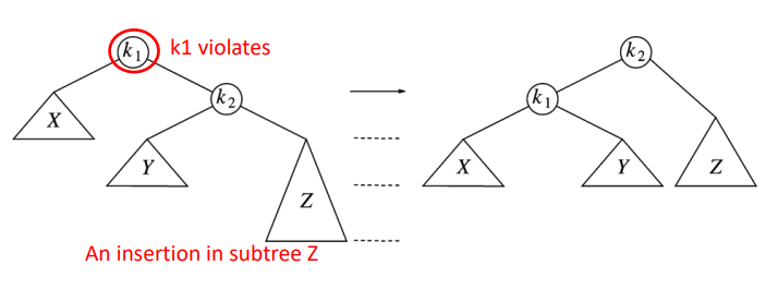
=> 시간 복잡도
insertion : O(log2n), single rotation : O(1)
double rotation
- LR insertion
- RL insertion
지그재그 모양으로 insertion이 이루어지는 경우
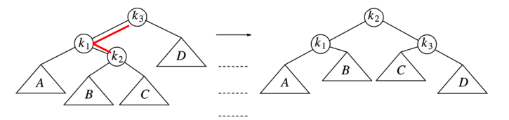
Left right는 가장 말단 노드를 root로 올린다.
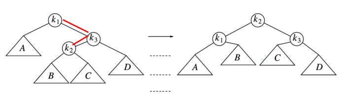
right left insertion도 말단 노드를 root로 올려서 해결한다.
> B-Trees (39~59)
<motivation>
데이터베이스나 파일 시스템에서 많이 사용한다.
큰 데이터셋에 대해서는 메인 메모리에서만 처리하기는 어렵다.
디스크에 저장하는 경우, 메인 메모리와는 다른 접근법을 취하여야 한다. => 더 많은 branch를 허용해서 트리의 높이를 줄이기!
<mulati-way B-Tree>
B-Tree는 자식 노드의 개수가 2개 이상인 트리를 말한다.
B-Tree는 m-way라고 해서 어떤 값의 children도 가질 수 있다.
rule 0. root node는 0개 혹은 적어도 2개 이상의 children을 갖는다
rule 1. root나 external node를 제외한 노드들은 ceil(m/2) 이상 m 이하 개의 children을 갖는다
rule 2. external node의 깊이는 모두 동일하다
rule 3. internal node의 key 개수 : children -1 / external node의 key 값 : ceil(m/2)-1~m-1
'Computer Science > 자료구조' 카테고리의 다른 글
| 자료구조 | Shortest Path and Activity Network (0) | 2022.01.09 |
|---|---|
| 자료구조 | binary trees, heap sort, threaded binary trees (python 구현) | Trees (0) | 2022.01.08 |
| 자료구조 구현 | selection sort, bubble sort, insertion sort, shell sort, quick sort (python 구현) | 정렬 (0) | 2022.01.08 |
| 자료구조 | Shortest Path and Activity Network | 숙명여대 학점교류 (0) | 2022.01.07 |
| 자료구조 | Graph | 숙명여대 학점교류 (0) | 2022.01.07 |